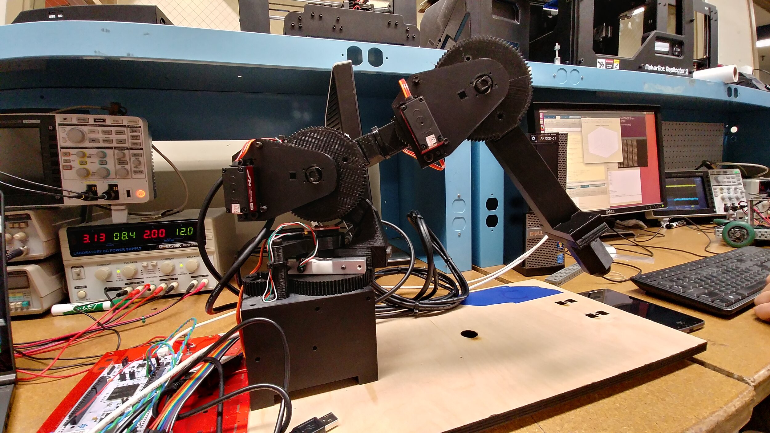
The 3D printed 3 degree of freedom robotic arm on its base

Summary

I worked on this project with two teammates. It was the culmination of work done with kinematics, force sensing, and manipulation using a 3-DOF robotic manipulator. The goal of this project was to sort objects in the robot’s workspace by weight and color using strain gauges and computer vision. First, the gauges were calibrated to return accurate values of the torque at each joint of the arm based on the unique properties of the arm and a provided scaling factor. Then, the camera was configured to search for three colors of objects in the workspace based on their size and Hue, Saturation, and Value (HSV) parameters. In order to pick up objects, a gripper was attached to the end of the manipulator and programmed to open or close based on a command sent to the micro-controller's firmware. Finally, using a state machine and trajectory generation programs we had developed, the arm picked up and sorted objects based on the color and weight information gathered during the process.

System Architecture and Joint Level Control

The first step of this project was to configure our robotic arm to respond to an SPI Interface, and then tune the arm’s PID controller. We developed a serial communication protocol to send commands to the controller and log data to the computer in real-time. The data was recorded and plotted via MatLab. PID gains were tuned iteratively using the data we gathered until the arm had low overshoot, minimal steady-state error, and quick rise time.

Hardware and Software

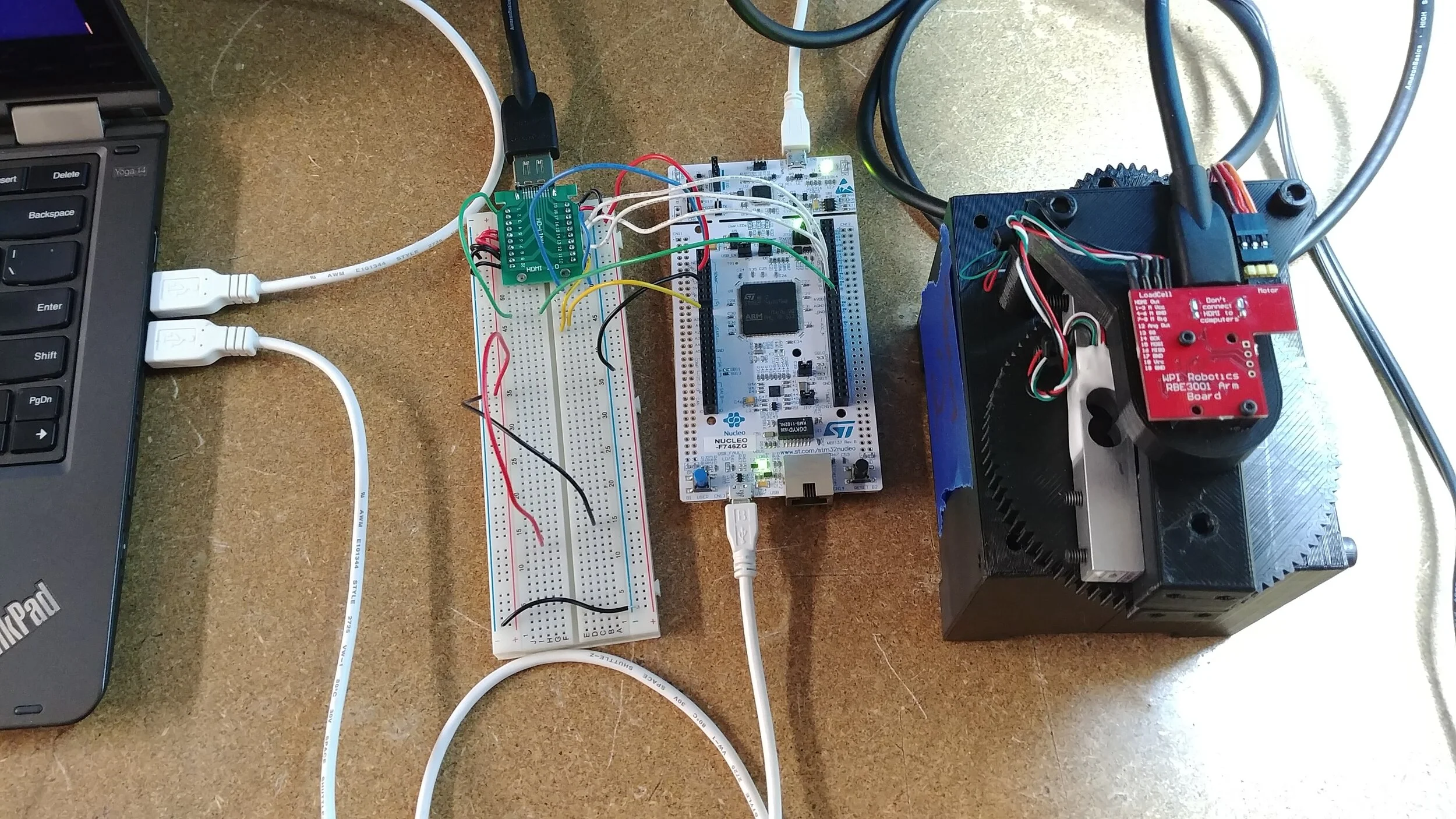
The Nucleo-F746ZG development board was used in conjunction with Mbed OS as the central platform for this project. The base/shoulder link of a 3-DOF robotic arm was attached to the Nucleo via a breakout board. The arm was equipped with force and position sensors. The primary task for this stage of the project was to move the shoulder link to a desired setpoint using PID control while modeling and storing the real-time angular position in MatLab. This task requires a working communication protocol, live data transfer, a working virtual model, and tuned PID gains. Each of these sub-tasks requires an understanding of the C++ firmware, MatLab scripting, and the hardware and datasheets for the Nucleo and peripherals.

Communication Protocol

We established a communication protocol to send and receive data from the Nucleo via Matlab. 64 bytes of data could be sent synchronously from the Nucleo to the breakout board and vice versa using the SPI protocol. This corresponded to sixteen 32-bit floating point integers, which was enough room for all of the necessary data to be transferred. The communication protocol was designed in C++, where packets of data were read, written, and transferred between the Nucleo and the breakout board. In MatLab, the status command was sent, and the status packet received and parsed, according to the protocol. The values of three encoders (shoulder, elbow, and wrist) were received and decoded using this protocol. PuTTY was used to view the serial output values of the encoder. During this stage we also created a home position for the arm using baseline encoder values and an offset constant. These values were hardcoded into the firmware as an offset in the PID calibration procedure.

A DAC output was implemented on the Nucleo that mapped the angle of the axes of each arm such that the range of the DAC comprised the full range of motion of that link. This was accomplished by adding 1300 to the encoder value (ticks) to produce a positive value, then scaling 2500 ticks to 3.3V (the maximum analog output), thus mapping -1300 ticks to 0V, and +1200 ticks to 3.3V. The DAC output was updated with each iteration of the servo loop (and encoder read) by placing the update within the body of that loop. The DAC output was tested by connecting it to an oscilloscope in order to assess the step response and tune the arm.

PID Tuning

The link was controlled by a PID control loop. To tune the PID gains, the Proportional, Integral, and Derivative terms were originally set to zero. First the P gain was slowly increased until the link was able to reach the setpoint with minimal overshoot. Once the P gain was tuned, the I and D gains were increased to dampen the oscillation of the link at the setpoint.

Originally our PID gains were much less responsive than the default settings, taking over 200 microseconds to respond. The default PID tuning responded to the setpoint in approximately four microseconds. After adjusting the PID gains, we were able to reduce the rise time to half of the default time. This can be seen in the figure to the left.

The top half of the figure shows the rise time of the link as it responds to a setpoint using the default PID values. The bottom half of the figure shows the rise time of the link using our tuned PID values. Not only is the response time better for our link, our PID tuning demonstrates no bounce at the setpoint, unlike the default PID tuning, which results in slight overshoot and correction.

We also tested the accuracy of our PID controller. First, we manually set the arm to an arbitrary angle. We read the raw encoder value of the arm using PuTTY, and used this as the setpoint for the arm. Leaving the power off, we moved the arm away from the setpoint. We then powered on the arm, and once it settled at the setpoint, read the raw encoder values with PuTTY. The PID controller was able to move the arm to less than one tick away from the setpoint in three trials.

We created a live model of the link using MatLab to show the arm position and path traveled in 3D and in real time. Using a timed loop, the MatLab program requested a Status packet from the robot. This packet contained the current encoder value for each joint. To transform the encoder tick value to an angle we compared the encoder ticks read from PuTTY as the link was turned 90 degrees, using a protractor as reference. The number of encoder ticks per degree was calculated to be 12. We wrote a function to plot the angle of the link as the degree values were calculated. This function created a plot in MatLab, calculated the cartesian coordinates for a point one unit from the origin at the given angle, and refreshed the plot with each new encoder value. The angle values from the encoder were recorded in a .csv file.

I especially enjoyed working on the modeling aspects of this project, so I volunteered to program most of the functionality for the 3D model. The program takes the lengths of links 1 and 2, as well as points representing the elbow and tool tip, and generates a three dimensional plot with a stick model of the arm. Because all three links of the arm are the same length, for simplicity’s sake I made them all equal to one.

To plot the position of each link, a vector was created representing the start and end point of each link in 3D space. A point v0 = [0 0 0] was created for the origin. The first link is the rotating base, which has an endpoint v1 = [0 0 1]. Vectors were constructed linking the start and endpoints of the links of the arm for each cardinal direction. With vectors for each link calculated, a plot was constructed to show the position of each link in the system. To add clarity to the 3D plot, circles showing the maximum range of the arm along each cardinal direction were plotted from the origin. A ‘shadow’ was added by plotting the xy projection of links 1 and 2 onto the xy plane of the plot, which gave the model a better sense of depth. The figures below show examples of the robot at the given encoder setpoint with a corresponding live 3D model.

Link-over-time (1).jpg — Control and Trajectory Generation

There are two types of kinematic equations used in the control of this robot: forward and reverse. Forward kinematics are used to find the arms position in task space based on the joint parameters. For example, if you know the angle of the three joints, you can use forward position kinematics to determine the (x,y,z) position of the end-effector. Inverse kinematics are useful for the opposite; when the (x,y,z) position of the end-effector is known, inverse kinematics can be used to find the joint parameters necessary for the robot to be in that configuration.

Forward Position Kinematics

Forward position kinematics for the robot are derived from the frame transformations from the base to the end-effector using D-H Parameters. The figure to the right demonstrates the coordinate frames for the 3 DOF robotic arm as it was configured for this project.

D-H Parameters are a method of describing the transformation from one reference frame to the next, which allows the motion of the individual links to be calculated relative to each other and propagated throughout the entire system. There are four D-H Parameters.

‘α’ represents the angle between the preceding z axis and the following z axis.
‘a’ is the distance the origin of the succeeding frame is translated along the x axis of the preceding frame.
‘d’ is the distance the origin of the succeeding frame is translated along the z axis of the preceding frame.
‘θ’ is the angle between the preceding x axis and the following x axis.

For example, using the figure to the right:

The z axis for frame 1 is rotated 90° relative to the z axis of frame 0, so the corresponding D-H Parameter ‘α’ is 90°.
The z axis of the frame (x1,y1,z1) is not translated along the x axis of the frame (x0,y0,z0), so the D-H Parameter ‘a’ is 0.
The origin of reference frame (x1,y1,z1) is translated a distance l1 from the base reference frame (x0,y0,z0), meaning the D-H Parameter ‘d’ is equal to l1.
The x axis is rotated a variable amount q0 based on the angle of the first joint, corresponding to the D-H Parameter ‘θ’.

The D-H Parameters are plugged into a 4x4 transformation matrix that captures the rotation and position changes from one reference frame to the next. The transformation matrices are multiplied together to create the full forward position kinematics transformation matrix. These calculations were performed in MatLab while the robot was running, which allowed us to model the arm in real time. These calculations were also used to find the manipulator Jacobian Matrix, which was used for force sensing.

Inverse Position Kinematics

Inverse position kinematics are used to determine the joint angle values from the position of the end-effector in (x0,y0,z0) task space. This calculation was made easier by treating the second and third links of the 3 DOF arm as a planar 2 DOF system, with the plane moving based on the first link. The figure to the left shows the robot in profile, which is useful to demonstrate the planar analysis.

The first step in deriving joint values from task space coordinates was calculating the radius, ‘r’ in the figure to the left. The radius is the vector from the origin to the (x0,y0) position of the end-effector. The angular position of the plane (and of the first joint), represented by q0 in the figure above, is the inverse tangent of the (x0/y0) coordinates.

With these values the second and third links can be treated as a two degree of freedom arm. The angle of the elbow joint (q2) was calculated first, then the angle of the shoulder (q1) was calculated.

There were many locations for the end-effector in the workspace where the robot could have used an ‘elbow-up’ or an ‘elbow-down’ position. In these cases our program first checked to make sure that the arm would not be set in an impossible position where the base of the robot, the ground, or another obstacle would prevent it from reaching its location. We also built in failsafes to prevent the robot from attempting to reach setpoints outside of its workspace and to catch any imaginary values that might be returned during the calculations. We avoided these conditions using try-catch statements that would activate recovery behavior or alert us that something had gone wrong.

Trajectory Generation

We created MatLab functions to generate trajectories for the arm using a cubic polynomial equation. A cubic polynomial is useful in this case because it accounts for control of the position, velocity, and acceleration of the arm as it moves to a setpoint. The robot’s motion within the workspace was between setpoints that were given in (x0,y0,z0) coordinates. Our trajectory generator function used interpolation to create setpoints in between the initial and final setpoints to create a smoother path for the robot to travel. The graphs below show the position, velocity, and acceleration data for the arm as it travels from the home position to a setpoint (10,5,15).

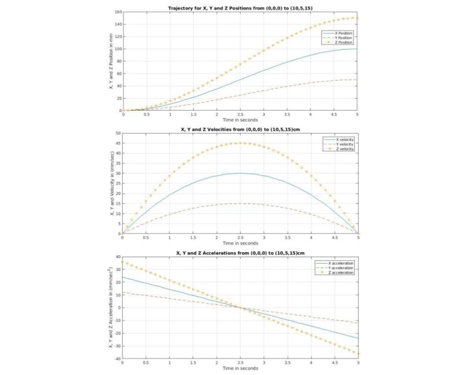
It is clear that the position of the end-effector, shown in the first graph, follows a cubic trajectory from the home position to the setpoint. This is the desired behavior because it represents a smooth motion. The acceleration of the end-effector, shown in the third graph, is linear. This means that the arm accelerates from rest to its maximum velocity and then decelerates back to rest as it approaches the goal setpoint. If the robot was traversing a larger workspace or doing longer maneuvers, a higher order polynomial would have been desired to allow control of the acceleration of the arm. This was not necessary for the scope of this project.

One of the most interesting parts of this project for me was adding a camera to this system. The camera allowed the robot to observe its workspace and interact with the objects placed in the workspace in really interesting ways, and it was something I hadn’t done before. I was very excited to add image processing functionality to this project. At this stage in the project, the robot could move itself to a setpoint anywhere within its workspace using a smooth cubic trajectory, but we were still hardcoding in setpoints for the robot to move to. After adding in computer vision, the robot was able to sense objects in the workspace and sort them based on their color. We used the MatLab to process the images taken by the workspace camera. Throughout the program loop, the camera would capture a picture of the workspace, which was then sent through a series of filters to process the image to be usable by the program to determine a setpoint for the arm. The figures below show the steps in the image processing program.

This is the ‘raw’ image captured by the workspace camera. A lot of the image is outside the workspace, which is both unusable and can create false positives later in the process. The blue tape at the top of the image represents the edge of the robot’s workspace. The red ball is the target object for the arm. the black circle is a hole in the center of the workspace where the robot places the end-effector in the home position. The eight black dots around the center of the workspace are used to calibrate the camera

In the second stage of the process the image is cropped down to remove unnecessary, non-workspace parts of the image.

After testing multiple color spaces in the MatLab Color Thresholding application, we settled on HSV because it returned the most consistent results. HSV, or Hue-Saturation-Value, allowed us to precisely select the color we wanted to filter without noise and with good tolerance for the different light conditions that could be found in the lab depending on the time of day or the weather.

In this example, the red filter was used, which has filtered out everything except the red ball and the power cord to the right. We eliminated false positives from outside the workspace by further cropping the image within the program. During this project the robot would look for red, blue, green, and yellow balls; so a threshold filter was created for each of those colors. Each of the color filters had to be tested on multiple days and at different times of day to ensure that the program had enough tolerance for different lighting conditions.

Next the image was turned into a grayscale image, and then a binary image, as seen on the left. A binary image contains pixels that are either white or black. This makes it much easier for the program to detect edges.

Binary images could still contain unwanted noise, however, so two filters were used to remove unwanted noise and false positives. An area filter was used to crop off areas that were outside the workspace and a size filter was used to remove objects with an area of less than 60 pixels.

With a clean binary image the program can create a centroid with relative ease. The centroid of the ball is used to create a setpoint for the robot so that they can be picked up and sorted.

In the final iteration of this project the camera was used to detect a dynamic number of objects at random positions in the robot's workspace. The camera would capture a still image at the beginning each loop of the sorting operation. The program would use the color filters to find the location and number of objects in the workspace, then process the image to find the centroid of each object. The robot would then generate a trajectory from its current position to the centroid of one of the objects. Once it had reached the object the robot’s end-effector would grab the object and sort it based on color and weight.

Each link of the robot was equipped with a strain gauge that allowed us to measure the amount of force being applied to its end. These sensors were necessary to be able to sort the objects in the workspace by weight. We wrote a MatLab function to transform the force from joint space to task space using the transpose of the Jacobian. These readings were smoothed with a rolling average in the robot's firmware to ensure a steady and accurate tip force vector. As can be seen in the figure above, we added a vector to the live MatLab simulation (shown in blue) that would visualize the amount of force a the tip of the end-effector.

To reduce noise while weighing objects in the workspace, the robot moved into the configuration shown in the simulation above, with the second link raised to be in line with the first link, and the third link at a right angle to the second link. This configuration resulted in the least noise. The figures below show the force vector while the robot is holding an object and while the robot is not holding an object. The force vector’s length corresponds to the magnitude of the force. This makes it easy to see in the simulation approximately how much weight the robot was holding. Based on this measurement the robot could sort the objects by weight.

Force vector with robot holding an object.

Force vector while the robot is not holding an object.

Results

This project synthesized sensing of both the robot and its workspace to create a dynamic system capable of responding to its environment in real time. We created a motion control program that used a cubic polynomial to ensure smooth trajectories from start to setpoint and position kinematics to update a live simulation of the arm for the operator. Using a camera the robot was able to detect objects entering the workspace. Following image processing the robot was able to travel to the objects, pick them up, and then sort them. Sorting was accomplished using color masking filters in the HSV colorspace and strain gauges on the robot’s arm to measure the force applied at the end-effector.

Overall this project was a great success and I had a lot of fun working on it. I had the opportunity to try out new techniques of sensing both on the robot using strain gauges and encoders and off the robot using a camera. This was my first foray into computer vision and image processing and I really enjoyed testing out filters in different color spaces to find one that was both precise and robust. If you’d like to learn more about this project’s technical details, check out the report we wrote below:

Final Report (PDF)

Three Degree of Freedom Robotic Arm